
Welcome to our Tips & Tricks page!
A space where we share quick insights, methods, and good habits with data scientists.
Good data science isn’t just about models or fast algorithms. It’s about the choices we make before, during, and after the analysis, and about the questions we ask along the way. Asking the right question is often the hardest and most valuable part of the work.
Good analysis comes from curiosity, attention, and flexibility.
Enjoy your reading!
Tip 01 — Take it easy with preprocessing

Sometimes data scientists go a little too far with preprocessing! A frequent mistake is to transform the response or the covariates just because their histograms don’t look Gaussian.
That’s wrong, and it can even be misleading.
The normality assumption in regression does not concern the marginal variables, the distribution of the errors, and therefore, \(Y\mid X_1 \ldots X_p\), where \(p\) is the number of predictors.
What truly matters is whether the residuals behave approximately like Gaussian, once the model is fitted. A non-Gaussian \(Y\) or \(X_j\) (\(j=1,\ldots p\)) tells us very little about it.
Preventive transformations are rarely help and often distort what matters. Fit the model first, inspect the residuals, and then decide if a transformation makes sense.
Let’s give a look to an example.
Consider the following Data Generating Process:
\[
\left\{
\begin{aligned}
X_{1i} &\sim \mathrm{Ber}(\pi),\\
X_{2i} &\sim \chi_1^2,\\
Y_i &= \beta_0 + \beta_1 X_{1i} + \beta_2 X_{2i} +
\varepsilon_i,\qquad \varepsilon_i \sim N\!\left(0,\tfrac{1}{4}\right),
\; i=1,\dots,n.
\end{aligned}
\right.
\]
with \(\beta_0 = 0\), \(\beta_1 = -3\), and \(\beta_2 = 1.5\).
All the assumptions for a linear regression model are perfectly satisfied here, as the errors are normal distributed and independent of the predictors.
Scary, isn’t it? Don’t worry, just fit a linear model and check the residuals! Here is what it comes out:
Call:
lm(formula = Y ~ X1 + X2)
Residuals:
     Min       1Q   Median       3Q      Max
-1.33657 -0.31524  0.01153  0.30351  1.56493
Coefficients:
            Estimate Std. Error t value Pr(>|t|)
(Intercept)  0.03545    0.03938    0.90    0.369
X1          -3.05142    0.04826  -63.23   <2e-16 ***
X2           1.48158    0.01627   91.09   <2e-16 ***
---
Signif. codes:  0 '***' 0.001 '**' 0.01 '*' 0.05 '.' 0.1 ' ' 1
Residual standard error: 0.482 on 397 degrees of freedom
Multiple R-squared:  0.9687,    Adjusted R-squared:  0.9685
F-statistic:  6140 on 2 and 397 DF,  p-value: < 2.2e-16
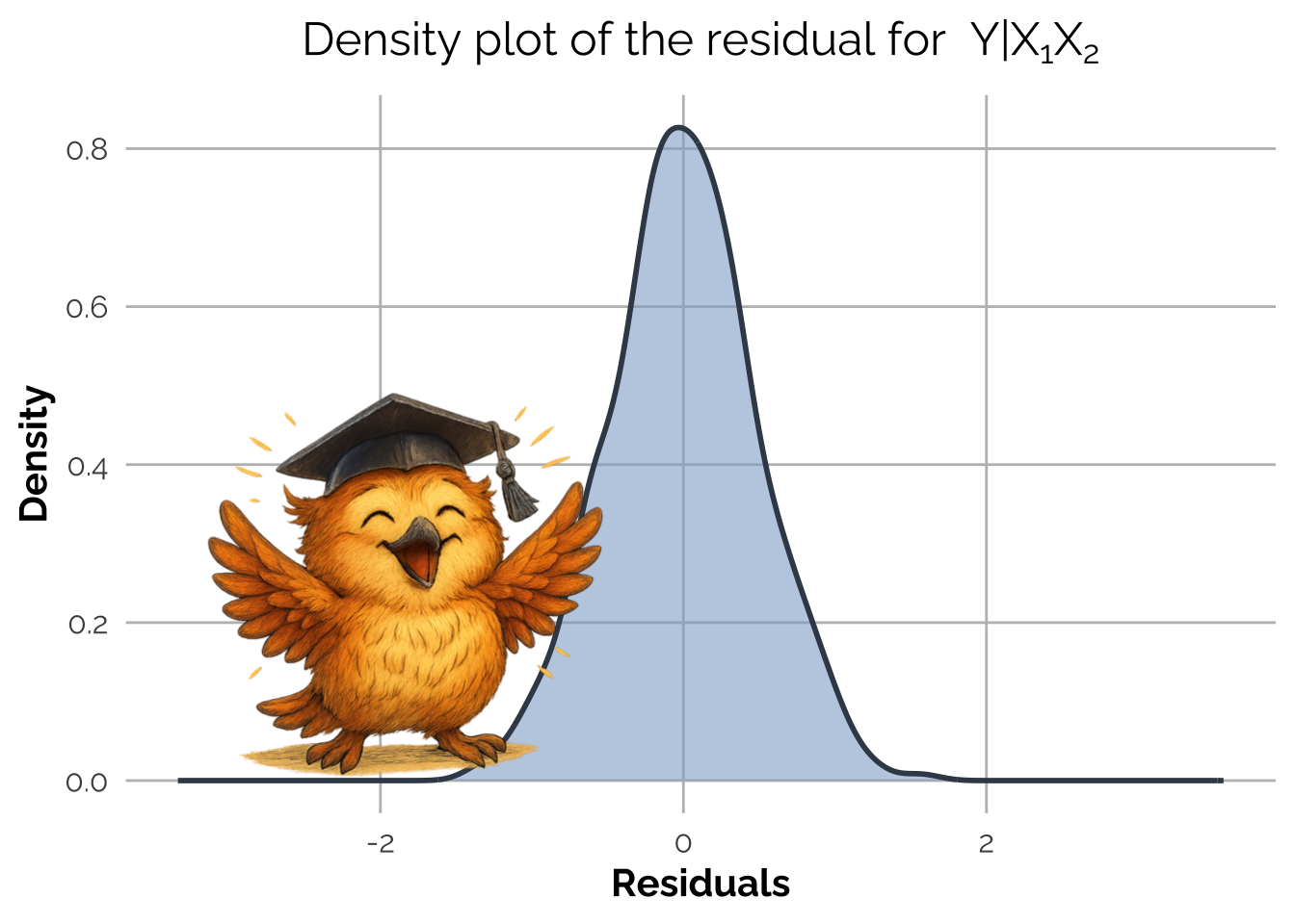
The summary appears ok and look at the plot of the residuals! They are Gaussian, as expected from the Data Generating Process.
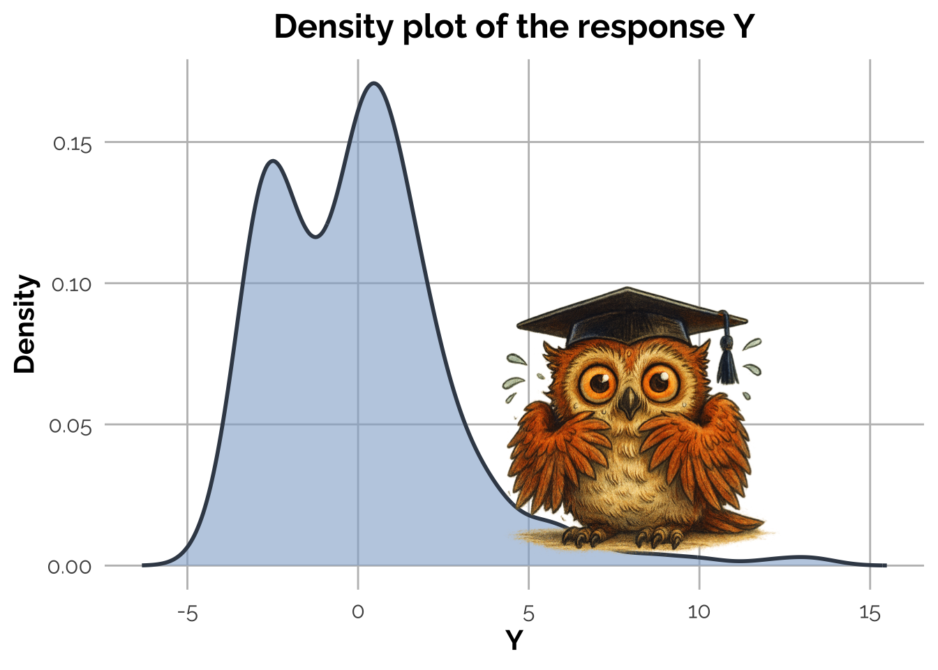
A common mistake would have been to transform \(Y\) or \(X_2\) because they did not appear normally distributed, because of the skewness on the marginal histogram/density plots.
It would have been a mess!
Let’s do a test to see if this is true. Imagine we had panicked after seeing the skewed histogram of \(Y\) and \(X_2\), and decided to fix it with a log transformation. That’s a typical preprocessing overreaction — and here’s the result where \(Y^*_i = \log(Y_i – \min(Y) + 1)\) and \(X_{2i}^* = \log(X_{2i})\).
Call:
lm(formula = Y_log ~ X1 + X2_log)
Residuals:
     Min       1Q   Median       3Q      Max
-0.81084 -0.14946 -0.04069  0.12247  0.96413
Coefficients:
             Estimate Std. Error t value Pr(>|t|)
(Intercept)  2.044469   0.019919  102.64   <2e-16 ***
X1          -0.622621   0.026167  -23.79   <2e-16 ***
X2_log       0.142818   0.006458   22.11   <2e-16 ***
---
Signif. codes:  0 '***' 0.001 '**' 0.01 '*' 0.05 '.' 0.1 ' ' 1
Residual standard error: 0.2611 on 397 degrees of freedom
Multiple R-squared:  0.7356,    Adjusted R-squared:  0.7343
F-statistic: 552.3 on 2 and 397 DF,  p-value: < 2.2e-16
The fitting is actually worse, with R-squared decresd from (0.9687) to (0.7343)!
Let’s see what happens to the residuals.
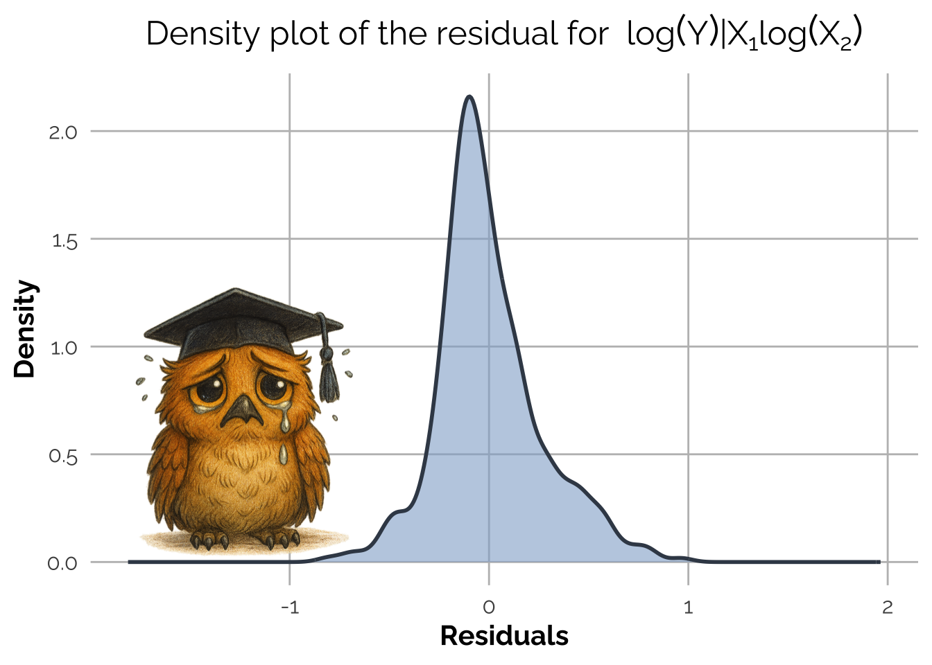
They are so much worse, right? After the transformation, the residuals are no longer Gaussian and the model coefficients are not close to the true ones. By transforming \(Y\) and \(X_2\) we’ve broken the linear relationship present in the Data Generating Process.
Takeaway:
If it’s not broken, don’t fix it. Check the residuals, not the marginals.
Curious about what to check after residuals? Stay tuned for future posts!